Assembling the Trajectory Parameters
In the previous section, we noted that many modern bullets have velocity versus distance profiles that can be described by Eq 1 with V being the velocity versus range S, Vz the least squared adjusted muzzle velocity, and A and B are fitted constants. The B term is the drag term, and we can call the A term a drag modifier.
V(S) = A S^2 + B S + Vz = (A S +B) S + Vz (1)
Transit Time T(S)
Setting V = dS/dT, with R = sqrt(4 A Vz -B^2) and of necessity real, we integrate (see note) to get the transit time to range S
T(S) = 2/R atan( (2 A S + B)/R) + Cint (2)
Since T(0) = 0, we can find Cint and an equation for the time to go from zero to distance S is:
T(S) = (2/R) (atan( (2 A S + B)/R) - atan( B/R) ) (3)
If (4 A Vz - B^2)is negative, we need different math from Eq. 2. Bullets for which (4 A Vz - B^2) is negative have a rapid increase in the drag and
often do not fly well. Eq. 16 is also a possible option, but the exponential should be fitted to the data directly rather than using the B term as a bridge.
Eq. 15 might also be used generally if the parabolic relation fails.
Sighting Angle
So now we have a closed form for the transit time T as a function of horizontal distance S. Again note this expression is no better than the accuracy of Eq. 1.
Once it leaves the barrel, the gravitational drop of a bullet fired horizontally is (1/2)G T^2. If the gun is not horizontal but at an angle a radians, small enough that sin(a )= a, the initial velocity will include a vertical component a Vz.
Then the vertical position E of the bullet relative to the barrel, (+ for up) at time T will be, where G is the acceleration of gravity.
E (S) = a Vz T(S) - (1/2) G T(S)^2 (4)
This expression is relative to the barrel. To make it relative to a sight above the barrel, correct for scope axis offset from barrel axis P.
E ( S) = a Vz T(S) - (1/2) G T(S)^2 - P (5)
For hitting a bullseye at distance Sz with a scope above the barrel a distance P, we set E(S)= 0 and solve for a, the angle between the barrel and the scope, in eq. (6).
a = (P + (1/2) G T(Sz)^2 )/ (Vz T(Sz)) (6A)
This a is in radians. Multiply by 1000 to get mils and by 60*180/pi to get minutes of arc (MOA). Use this equation and resulting a's to change target distances using the clicks on the scope. This equation is adequate for Sz in the 10's of yards, but may require drag adjustment for hundreds of yards. A possible modification is shown later in the paragraph on Finite Difference Equations.
Apex and S(T)
The apex of the trajectory is when the vertical velocity goes to zero dE(S)/dT=0, that is:
aVz = G T(S) (7)
T= aVz/G (8)
Setting (3) to (8) and solving for S using still R = sqrt(4 A Vz -B^2) gives
S(T)= R/(2A)[ tan( RT/2 + atan(B/R) ) -B] (9)
Apex distance = (R/ 2A) tan( a R Vz/ 2G + atan(B/R)) - B/2A (10)
The apex will be the highest point on the trajectory of a horizontal fire. Knowing it is useful for finding point blank ranges. The apex does not
explicitly depend on the scope offset though a does. Some drag correction might be in order, but we will neglect it.
Maximum Useful Ranges
As the velocity of bullets drop into the subsonic range they tend to become unstable, or at least relatively more rapidly lose remaining velocity. From the fitting parameters we can find the range for this to happen.
Useful Range = (-B - sqrt(B^2 - 4 A (Vz-1200))/ 2A (11A)
In addition there is a matter of the overall accuracy of both Eq. 1 and the drag corrections to follow. Insofar as the retrofit of eq 1 to the data is as accurate
as the data, 11A is sufficient. When failure of eq. 1 to match the data begins to occur, keep in mind another approximation to the useful range:
Accurate Range = (-B - sqrt(B^2 - 2A VZ))/ 2A (11B)
Corrected Gravitational Bullet Drop
Without including drag and air viscosity effects, the drop at time T of Newton's apple or a cannon fired horizontally is
Drop of apple = .5 G T(S)^2 (12A)
where G is the acceleration of gravity, 32.17 ft/sec^2 at the equator, and 0.44% more at the poles.
But a bullet falls more slowly than Eq. 12A suggests for complicated aerodynamic reasons. Most of the slowing is due to the same drag effect that slows the bullet along its aim path. McCoy (ref. 2) gives interesting correction functions to the vertical drop distance of Eq 12A. The McCoy correction assumes the same drag for drop as for forward motion, which assumption may not be always valid. A surprisingly accurate average of all three of the McCoy drop corrections is the term (V(S)/Vz)^ 0.3 .
Assuming that the same drag applies to drop as to horizontal motion, and including the offsets due to scope and barrel angle gives the final total
drop (perhaps incorrectly using negative as "down")
Drop = ( a T Vz - P - .5 G T(S)^2 ) (V(S)/Vz)^0.30 (12B)
In the event that the drop given by 12B is not enough, we can apply a correction H to 12b, and add a term (1-H)* .5GT^2.
H corrected Drop = ( a T Vz - P - .5 G T(S)^2 ) (H (V(S)/Vz)^0.30 +(1-H) ) (12C)
As written, H of 1 is full correction, with the drop moving toward pure gravitation as H is decreased.
The H correction does depend on the bullet so H will move around with the bullets used. After adjusting H to match data at, say, 500 yds with this correction we may still be off by 2 moa at 800 yds. The function is in lieu of a more accurate method described in the paragraph on "Drag and the Point Mass Approximation". The drag correction multiplier H is the fourth number needed to describe drop tables.
Summary of Equations For a Pretty Good Drop Table
Find the parameters A,B and C=Vz for Eq. 1 and check goodness of fit. Around Mach 2.5 they should be within a few 1/10 percent or so.
Evaluate your useful distances.
Measure your sight offset P and choose the sight zero distance Sz. Find tilt angle a in Eq. 6.
Starting at zero, incrementing in steps of 50 yds, calculate the flight time T, then
Find velocity V (eq. 1) , S/Vz for wind estimates, and the Drop, eq. 12 B.
The wind distance offset estimate is (S/Vz-T) * (wind speed), discussed in the section on variation.
Full Accuracy Finite Difference Equations for Drag Corrected Drop
The starting point for external ballistics is often the equation
dV/dT = -CMcC V V McCoy (Ref. 2) Eq 5.8
where CMcC is the raw drag coefficient, V is the velocity vector, V is the magnitude of the vector, and T is time. From the definitions we can get to
dV/dT = (dV/dS) (dS/dt) = V (dV/dS)= -CMcC V^2 13A
By decomposing the velocity vector into x and y components and including the acceleration of gravity
for the Y component:
dVy/dT = -CMcC Vx Vy - G McCoy Eq. 5.9
By including dVx/dT = V (dVx/dS) and the velocity profile, the vertical acceleration is:
dVy/dT = (A S^2 + B S + Vz) Vy - G 14
This assumes the drag for vertical motion is the same as that for horizontial.
At S= 0, the initial Y is -P, the sight offset. The initial Y velocity is the sight angle (or its tangent) times the muzzle velocity.
As with the non iterative method, we start the calculation at zero range then step in distance. At each step calculate the time, acceleration, delta velocities and delta distances step by distance step. A reasonable interval is 1/4 foot, but even shorter steps may be needed for full accuracy.
For this more accurate calculation, a better estimate of the sight angle a is needed. One possibility using Ts = T(Sz) is
a = (P + .5 G Ts^2) / (Ts ( .78 Vz + .22 *V(Sz))) 6B
There are better approximations for (a) to be explored, but using 1/4 foot interval and eq. 6B a sampling of various bullets gives roughly 1 inch accuracy at 1000 yds.
Decoupling of X and Y Velocities
Anyone who wants to reproduce the steps noted below should consider becoming familiar with Xmaxima and Wolfram/alpha.com on the internet.
The vertical velocity which gets numerically integrated comes from McCoy's eq. 5.22
dVy/dx = - CMcC Vy - G /Vx. McCoy 5.22
Inserting McCoy 5.21 into 5.22 gives the following relation between the Vx and Vy functions.
Vy dVx/dX - Vx dVy/dX = G BD1
Recognizing the parallel between BD1 and the equation for the derivative of the ratio of two functions, we can write
d/dx (Vy/Vx) = -G/Vx^2 BD2
Given an expression for Vx, either an analytical approximation or a curve fit, we can integrate to find (Vy/Vx). For cases where we cannot find reasonable analytical expressions for the integral, we can use power series approximations.
Since we are interested in the drop, which is the integral of Vy dt, the integral for the drop is the integral of Vy (dx / Vx) so that
Drop(x) = integral( (Ci + integral ( -G /Vx^2 dx )) dx) BD3
where Ci is the constant of integration for the first integral which will provide the term (barrel angle)*range. The second constant of integration is the sight offset.
Validation of BD3 and Implications for Calcuations
Sierra Bullets provide tables of velocity profiles for their bullets for various Vz's. Allowing for variation in position, it is appears possible to adjust all the velocity data for each bullet to a single 6 term polynomial in position that fits a single profile to within roughly 2 parts in 10^5. Performing the double integration in BD3 at intervals of 4 per foot then gives drops within about one inch of the tabulated values at 1000 yds, Without knowing the origin of the published numbers it is hard to know what conclusions can be drawn from from this result, but the result supports the view that, to the extent velocity data can validate a particular drag function, the same data is sufficient for calculating trajectories.
Exact Drop Equation for Parabolic Velocity Profile
Eq. BD2 can be integrated then expanded in a Taylor series. The gruesome math is not produced here since there is little one can do without computer support to generate the executable code. The first term is by definition the (tangent of barrel angle)*distance . The second term is (1/2) G(distance/Vz)^2. Using 9 terms produces drops that are within 1/2 moa out to 800 yds for all bullets examined, now several hundred. The 9 term expansion seems accurate to within 1moa down to Mach 1 so long as the initial profile is accurate.
Exact Drop Equation for Exponential Velocity Profile
Now if we let CMcC= Q = r pi Cd / (8Cb) = d/ds ln(V) as in 13B and 13C for which r is air density, Cd drag coefficient, and Cb the ballistic coefficient, we can say that the horizontal velocity is approximately , where Vz is the muzzle velocity:
Vx = Vz exp(- Q X) BD4
Obtaining Q from tabulated velocity data is as easy as taking the ln of (slowest speed)/(muzzle speed) and dividing by the distance. It doesn't hurt to check a few intermediate points just to make sure the data is correct. Sometimes it is not. And you may be saying to yourself, "Hey, which is it? Is it exponential or parabolic?" The answer is "both and neither". The parabola fits the high velocity end of the velocity versus distance profile for many bullets. The exponential may be a better approximation when the velocity gets down to half or so of the muzzle velocity. As noted in the previous section, to describe the profile from Mach 3 down to mach 1 may take terms up to the 5th power of range. Note that the parabola is approximately the first two terms of the Taylor series expansion for velocity vs. distance fitted to the exponential. For now, we have no accurate approximation at the speed of sound and below, and the parabola is best at the high end.
So, making assumptions about Vx like BD4, and using BD 1 or 2 can we find an expression for Vy which can be integrated to find the drop? The answer is yes, with a bit of work. See BD8 below.
A boundary condition is that Vy has a term of the form (a Vz) where a is the muzzle angle. We can insert Vy = aVz + E(X) into BD1 and get an expression for E(X) and its derivative. Taking Laplace transforms, and solving for E(X) we can find an expression for Vy. It is rather a mess but whoever said it would be easy?
Vy = ( - a Q Vz - G/Vz ) exp(-Q X) (exp(2 Q X) -1) + a Vz exp(-Q X) (exp(Q X) -1)^2 + a VZ
------------------------------------------------------------- --------------------------------------------- BD5
2Q 2
where a is the barrel angle, G is gravity, Vz is muzzle velocity, X the range, and Q is the velocity profile constant.
BD5 is for the Y velocity as a function of range. To get bullet drop we must integrate this with respect to time, dt, but the time dimension is as defined along the trajectory. We can find time from distance per velocity, that is, we need the integral of
Vy[BD5] * dx/ Vx(x) BD6
Luckily XMaxima could handle this integral, for which the indefinite integral in Fortran follows. A picture of this eqn is below.
Drop= (a*VZ*((exp(2*Q*X)-4*exp(Q*X))/2. +Q*X)/Q/2 +(-a*Q*VZ-G/VZ) BD7
1 *(exp(2*Q*X)/2 -Q*X)/Q**2/2 +a*VZ*exp(Q*X)/Q)/VZ
Adding the term G/(4*Q^2*Vz^2) makes this integral exact at X = 0.
Note that BD7 is an exact expression for bullet drop in the context of the point mass approximation and an exponential velocity profile BD4, Note too that this approximation presumes the same drag coefficient both down range and due to drop, which approximation should be carefully considered.
To get the exact barrel angle for a particular sight distance with Newton-Raphson requires a bit more algebra but the convergence is rapid. For short distances a three term expansion should work with no iteration. Note that the derivative of BD7 wrt X is X. If anyone wants additional information, please email the address in the complaint section. Please be patient. The pay does not justify overtime.
Not comes the question, how good is all this for calculating trajectories? Using an iterative finder for the barrel angle, "sighting" at 100 yds, averaging the tabulated velocity ln(V)'s to get Q, for an arbitrary group of bullets we get the results in the table below. The largest error is 4 in. at 800 yds. for the .308, with all others 3 in or less. The column FIT(800) is the percentage error of the calculated velocity at 800 yds compared to the actual velocity. These data was chosen for comparison to BD7 because they included 1000 yd ranges and were on top of great stack of such data. Rifleist would be ecstatic to shoot as well as the computer does.
Calculated and Manufacturer Supplied Drop Using 100 Yd Zero
( C is calculated with BD7, D is from data sheets)
BULLET WT FIT(800) VZ 800Y(C) 800Y(D) 1000Y(C) 1000(D)
SCN 6.5X47 120 +4.0% 2772 197 198
SCN 6.5X47 139 +4.0 2690 190 188 344 342
SCN 6.5X55 108 +7.1 2950 176 173 329 328
SCN 308WIN 155 +5.9 2820 196 192 365 367
NAT 338LM 231 +4.5 3018 191 192
SCN 338LM 250 +3.1 2970 144 143 257 256
SCN 338LM 300 +1.8 2723 166 165 291 291
MEG 9.3X62 285 +0.4 2265 171* 173*
* IS FOR 600, NOT 800
Integrating BD2 to get Vy/Vx, for the exponential BD4 then integrating again to get y, produces the following drop equation, which so far seems to provide identical results to the cumbersome BD7.
Y = a*X - G( exp(2 Q X) - 2 Q X - 1)/(4 Q^2 VZ^2) BD8
In BD8, Y is the "drop", a is the tangent of the barrel angle, X is the range, G the gravitational constant, VZ is muzzle velocity, and Q is the velocity decay constant in the expression VX = VZ*exp(-Q X). BD8 should have a sight offset term added.
Other Forces: Coriolis, Centripetal, and Gravitational
For the point mass approximation it is relatively easy to find some correction for the lateral and vertical inertial forces. For comparison with other sources, we are trying to handle the reference frame acceleration (and gravity) written as 2 ( w X V) + w X (w X R) - G, where w is the angular rotation rate of Earth, X is the vector cross product, V is the vector velocity, and G is gravity. It is usual to call the first term the Coriolis acceleration and the second centripetal. Centripetal acceleration will result in velocity squared effects, and if there are no such terms, centripetal was not included. With today's precision and faster bullets this absence should be quite noticeable.
From BD2, the horizontal motion is fully decoupled from the vertical, and the Coriolis drift for flat fire in vacuum is McCoy's 8.52 : Drift to the right (in the northern hemisphere) = w range^2 sin(latitude) / Vz . Without having gone through the math, Rifleist suspects this will be accurate in air as well, based on the wind drift argument, that additional time spent in flight by the bullet will serve to acquire the local wind velocity and cancel out any Coriolis drift acquired during this time. For a 338 at 1000 yards, this is under 2 inches at 45 degrees north latitude, or about 2/3 % of the drop.
For the vertical component,we can embed all accelerations into the gravitational constant using the Eotvos acceleration, This can be done accurately only in an iterative calculation. The Eotvos effect on gravitational constant includes both Coriolis and centripetal terms: 2 w U cos(latitude) + ( (U- Ue) ^ 2 + v^2)/r where U is velocity to East, Ue is earths rotation speed (to the east, 1520 fps at the equator). This speed gives an acceleration at the equator of 0.11 fps^2.) , v is north to south speed, r the radius of the rotation which may depends on latitude. A bullet moving to the East experiences a lift and one moving to the West experiences increasing gravitation, until its speed gets to Ue. This is why it is expedient to launch rockets from Cape Canaveral rather than the West coast. It might suffice to use average velocity for the Coriolis term, and average square for the centripetal term. Using G = 32.26 and 32.08 in eq. BD7 to simulate comparative E to W and W to E firing, has the 250 grain 338 in the above table with Vz = 2970 and with 100 yd zeros showing a difference of 2" at 1000 yds. The average drop at 1000 yds is 256 in, so the inertial percentage is under 1%. With the flight time of 1.64 seconds the vacuum drops would be 517.7 and 520.6, and the McCoy correction is (v/vz)^.3 = .84
If your shooting precision is such that inertial effects are important, you should consider the value you use for G, variation of which could also have a noticeable effect as you move, say, from Texas to Canada. Gravity does change from 32.26fps^2 at the poles to 32.09 fps^2 at the equator. 0.11 fps^2 or .34% of this is due to centripetal force. Here in New Hampshire I get to use the average, 32.17 fps^2.
It would be very good to see some experimental verification of these calculations before making any life or death decisions using them. The notion of using gravitational constant to handle bookkeeping of the vertical inertial forces is interesting and is done by McCoy. Several authors make no mention of centripetal effects, yet as bullet speeds go up centripetal acceleration becomes relatively more important.
Neglected in this discussion is the change in vertical angle between the rotational center and the mass center in moving from the equator to a pole.
There is a video on the internet saying that the E-W/W-E Coriolis effect at 1000 yds is more than 6 moa. Rifleist suspects this is too high. It is mandatory that such portrayals include the shooters latitude and the direction of fire to be useful.
Whatever the calculation, if manufacturers would specify the conditions of their velocity measurements it would improve understanding of variation in shooting outcomes.
BD7 Drop equation is
In the previous section, we noted that many modern bullets have velocity versus distance profiles that can be described by Eq 1 with V being the velocity versus range S, Vz the least squared adjusted muzzle velocity, and A and B are fitted constants. The B term is the drag term, and we can call the A term a drag modifier.
V(S) = A S^2 + B S + Vz = (A S +B) S + Vz (1)
Transit Time T(S)
Setting V = dS/dT, with R = sqrt(4 A Vz -B^2) and of necessity real, we integrate (see note) to get the transit time to range S
T(S) = 2/R atan( (2 A S + B)/R) + Cint (2)
Since T(0) = 0, we can find Cint and an equation for the time to go from zero to distance S is:
T(S) = (2/R) (atan( (2 A S + B)/R) - atan( B/R) ) (3)
If (4 A Vz - B^2)is negative, we need different math from Eq. 2. Bullets for which (4 A Vz - B^2) is negative have a rapid increase in the drag and
often do not fly well. Eq. 16 is also a possible option, but the exponential should be fitted to the data directly rather than using the B term as a bridge.
Eq. 15 might also be used generally if the parabolic relation fails.
Sighting Angle
So now we have a closed form for the transit time T as a function of horizontal distance S. Again note this expression is no better than the accuracy of Eq. 1.
Once it leaves the barrel, the gravitational drop of a bullet fired horizontally is (1/2)G T^2. If the gun is not horizontal but at an angle a radians, small enough that sin(a )= a, the initial velocity will include a vertical component a Vz.
Then the vertical position E of the bullet relative to the barrel, (+ for up) at time T will be, where G is the acceleration of gravity.
E (S) = a Vz T(S) - (1/2) G T(S)^2 (4)
This expression is relative to the barrel. To make it relative to a sight above the barrel, correct for scope axis offset from barrel axis P.
E ( S) = a Vz T(S) - (1/2) G T(S)^2 - P (5)
For hitting a bullseye at distance Sz with a scope above the barrel a distance P, we set E(S)= 0 and solve for a, the angle between the barrel and the scope, in eq. (6).
a = (P + (1/2) G T(Sz)^2 )/ (Vz T(Sz)) (6A)
This a is in radians. Multiply by 1000 to get mils and by 60*180/pi to get minutes of arc (MOA). Use this equation and resulting a's to change target distances using the clicks on the scope. This equation is adequate for Sz in the 10's of yards, but may require drag adjustment for hundreds of yards. A possible modification is shown later in the paragraph on Finite Difference Equations.
Apex and S(T)
The apex of the trajectory is when the vertical velocity goes to zero dE(S)/dT=0, that is:
aVz = G T(S) (7)
T= aVz/G (8)
Setting (3) to (8) and solving for S using still R = sqrt(4 A Vz -B^2) gives
S(T)= R/(2A)[ tan( RT/2 + atan(B/R) ) -B] (9)
Apex distance = (R/ 2A) tan( a R Vz/ 2G + atan(B/R)) - B/2A (10)
The apex will be the highest point on the trajectory of a horizontal fire. Knowing it is useful for finding point blank ranges. The apex does not
explicitly depend on the scope offset though a does. Some drag correction might be in order, but we will neglect it.
Maximum Useful Ranges
As the velocity of bullets drop into the subsonic range they tend to become unstable, or at least relatively more rapidly lose remaining velocity. From the fitting parameters we can find the range for this to happen.
Useful Range = (-B - sqrt(B^2 - 4 A (Vz-1200))/ 2A (11A)
In addition there is a matter of the overall accuracy of both Eq. 1 and the drag corrections to follow. Insofar as the retrofit of eq 1 to the data is as accurate
as the data, 11A is sufficient. When failure of eq. 1 to match the data begins to occur, keep in mind another approximation to the useful range:
Accurate Range = (-B - sqrt(B^2 - 2A VZ))/ 2A (11B)
Corrected Gravitational Bullet Drop
Without including drag and air viscosity effects, the drop at time T of Newton's apple or a cannon fired horizontally is
Drop of apple = .5 G T(S)^2 (12A)
where G is the acceleration of gravity, 32.17 ft/sec^2 at the equator, and 0.44% more at the poles.
But a bullet falls more slowly than Eq. 12A suggests for complicated aerodynamic reasons. Most of the slowing is due to the same drag effect that slows the bullet along its aim path. McCoy (ref. 2) gives interesting correction functions to the vertical drop distance of Eq 12A. The McCoy correction assumes the same drag for drop as for forward motion, which assumption may not be always valid. A surprisingly accurate average of all three of the McCoy drop corrections is the term (V(S)/Vz)^ 0.3 .
Assuming that the same drag applies to drop as to horizontal motion, and including the offsets due to scope and barrel angle gives the final total
drop (perhaps incorrectly using negative as "down")
Drop = ( a T Vz - P - .5 G T(S)^2 ) (V(S)/Vz)^0.30 (12B)
In the event that the drop given by 12B is not enough, we can apply a correction H to 12b, and add a term (1-H)* .5GT^2.
H corrected Drop = ( a T Vz - P - .5 G T(S)^2 ) (H (V(S)/Vz)^0.30 +(1-H) ) (12C)
As written, H of 1 is full correction, with the drop moving toward pure gravitation as H is decreased.
The H correction does depend on the bullet so H will move around with the bullets used. After adjusting H to match data at, say, 500 yds with this correction we may still be off by 2 moa at 800 yds. The function is in lieu of a more accurate method described in the paragraph on "Drag and the Point Mass Approximation". The drag correction multiplier H is the fourth number needed to describe drop tables.
Summary of Equations For a Pretty Good Drop Table
Find the parameters A,B and C=Vz for Eq. 1 and check goodness of fit. Around Mach 2.5 they should be within a few 1/10 percent or so.
Evaluate your useful distances.
Measure your sight offset P and choose the sight zero distance Sz. Find tilt angle a in Eq. 6.
Starting at zero, incrementing in steps of 50 yds, calculate the flight time T, then
Find velocity V (eq. 1) , S/Vz for wind estimates, and the Drop, eq. 12 B.
The wind distance offset estimate is (S/Vz-T) * (wind speed), discussed in the section on variation.
Full Accuracy Finite Difference Equations for Drag Corrected Drop
The starting point for external ballistics is often the equation
dV/dT = -CMcC V V McCoy (Ref. 2) Eq 5.8
where CMcC is the raw drag coefficient, V is the velocity vector, V is the magnitude of the vector, and T is time. From the definitions we can get to
dV/dT = (dV/dS) (dS/dt) = V (dV/dS)= -CMcC V^2 13A
By decomposing the velocity vector into x and y components and including the acceleration of gravity
for the Y component:
dVy/dT = -CMcC Vx Vy - G McCoy Eq. 5.9
By including dVx/dT = V (dVx/dS) and the velocity profile, the vertical acceleration is:
dVy/dT = (A S^2 + B S + Vz) Vy - G 14
This assumes the drag for vertical motion is the same as that for horizontial.
At S= 0, the initial Y is -P, the sight offset. The initial Y velocity is the sight angle (or its tangent) times the muzzle velocity.
As with the non iterative method, we start the calculation at zero range then step in distance. At each step calculate the time, acceleration, delta velocities and delta distances step by distance step. A reasonable interval is 1/4 foot, but even shorter steps may be needed for full accuracy.
For this more accurate calculation, a better estimate of the sight angle a is needed. One possibility using Ts = T(Sz) is
a = (P + .5 G Ts^2) / (Ts ( .78 Vz + .22 *V(Sz))) 6B
There are better approximations for (a) to be explored, but using 1/4 foot interval and eq. 6B a sampling of various bullets gives roughly 1 inch accuracy at 1000 yds.
Decoupling of X and Y Velocities
Anyone who wants to reproduce the steps noted below should consider becoming familiar with Xmaxima and Wolfram/alpha.com on the internet.
The vertical velocity which gets numerically integrated comes from McCoy's eq. 5.22
dVy/dx = - CMcC Vy - G /Vx. McCoy 5.22
Inserting McCoy 5.21 into 5.22 gives the following relation between the Vx and Vy functions.
Vy dVx/dX - Vx dVy/dX = G BD1
Recognizing the parallel between BD1 and the equation for the derivative of the ratio of two functions, we can write
d/dx (Vy/Vx) = -G/Vx^2 BD2
Given an expression for Vx, either an analytical approximation or a curve fit, we can integrate to find (Vy/Vx). For cases where we cannot find reasonable analytical expressions for the integral, we can use power series approximations.
Since we are interested in the drop, which is the integral of Vy dt, the integral for the drop is the integral of Vy (dx / Vx) so that
Drop(x) = integral( (Ci + integral ( -G /Vx^2 dx )) dx) BD3
where Ci is the constant of integration for the first integral which will provide the term (barrel angle)*range. The second constant of integration is the sight offset.
Validation of BD3 and Implications for Calcuations
Sierra Bullets provide tables of velocity profiles for their bullets for various Vz's. Allowing for variation in position, it is appears possible to adjust all the velocity data for each bullet to a single 6 term polynomial in position that fits a single profile to within roughly 2 parts in 10^5. Performing the double integration in BD3 at intervals of 4 per foot then gives drops within about one inch of the tabulated values at 1000 yds, Without knowing the origin of the published numbers it is hard to know what conclusions can be drawn from from this result, but the result supports the view that, to the extent velocity data can validate a particular drag function, the same data is sufficient for calculating trajectories.
Exact Drop Equation for Parabolic Velocity Profile
Eq. BD2 can be integrated then expanded in a Taylor series. The gruesome math is not produced here since there is little one can do without computer support to generate the executable code. The first term is by definition the (tangent of barrel angle)*distance . The second term is (1/2) G(distance/Vz)^2. Using 9 terms produces drops that are within 1/2 moa out to 800 yds for all bullets examined, now several hundred. The 9 term expansion seems accurate to within 1moa down to Mach 1 so long as the initial profile is accurate.
Exact Drop Equation for Exponential Velocity Profile
Now if we let CMcC= Q = r pi Cd / (8Cb) = d/ds ln(V) as in 13B and 13C for which r is air density, Cd drag coefficient, and Cb the ballistic coefficient, we can say that the horizontal velocity is approximately , where Vz is the muzzle velocity:
Vx = Vz exp(- Q X) BD4
Obtaining Q from tabulated velocity data is as easy as taking the ln of (slowest speed)/(muzzle speed) and dividing by the distance. It doesn't hurt to check a few intermediate points just to make sure the data is correct. Sometimes it is not. And you may be saying to yourself, "Hey, which is it? Is it exponential or parabolic?" The answer is "both and neither". The parabola fits the high velocity end of the velocity versus distance profile for many bullets. The exponential may be a better approximation when the velocity gets down to half or so of the muzzle velocity. As noted in the previous section, to describe the profile from Mach 3 down to mach 1 may take terms up to the 5th power of range. Note that the parabola is approximately the first two terms of the Taylor series expansion for velocity vs. distance fitted to the exponential. For now, we have no accurate approximation at the speed of sound and below, and the parabola is best at the high end.
So, making assumptions about Vx like BD4, and using BD 1 or 2 can we find an expression for Vy which can be integrated to find the drop? The answer is yes, with a bit of work. See BD8 below.
A boundary condition is that Vy has a term of the form (a Vz) where a is the muzzle angle. We can insert Vy = aVz + E(X) into BD1 and get an expression for E(X) and its derivative. Taking Laplace transforms, and solving for E(X) we can find an expression for Vy. It is rather a mess but whoever said it would be easy?
Vy = ( - a Q Vz - G/Vz ) exp(-Q X) (exp(2 Q X) -1) + a Vz exp(-Q X) (exp(Q X) -1)^2 + a VZ
------------------------------------------------------------- --------------------------------------------- BD5
2Q 2
where a is the barrel angle, G is gravity, Vz is muzzle velocity, X the range, and Q is the velocity profile constant.
BD5 is for the Y velocity as a function of range. To get bullet drop we must integrate this with respect to time, dt, but the time dimension is as defined along the trajectory. We can find time from distance per velocity, that is, we need the integral of
Vy[BD5] * dx/ Vx(x) BD6
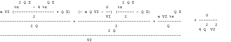
Luckily XMaxima could handle this integral, for which the indefinite integral in Fortran follows. A picture of this eqn is below.
Drop= (a*VZ*((exp(2*Q*X)-4*exp(Q*X))/2. +Q*X)/Q/2 +(-a*Q*VZ-G/VZ) BD7
1 *(exp(2*Q*X)/2 -Q*X)/Q**2/2 +a*VZ*exp(Q*X)/Q)/VZ
Adding the term G/(4*Q^2*Vz^2) makes this integral exact at X = 0.
Note that BD7 is an exact expression for bullet drop in the context of the point mass approximation and an exponential velocity profile BD4, Note too that this approximation presumes the same drag coefficient both down range and due to drop, which approximation should be carefully considered.
To get the exact barrel angle for a particular sight distance with Newton-Raphson requires a bit more algebra but the convergence is rapid. For short distances a three term expansion should work with no iteration. Note that the derivative of BD7 wrt X is X. If anyone wants additional information, please email the address in the complaint section. Please be patient. The pay does not justify overtime.
Not comes the question, how good is all this for calculating trajectories? Using an iterative finder for the barrel angle, "sighting" at 100 yds, averaging the tabulated velocity ln(V)'s to get Q, for an arbitrary group of bullets we get the results in the table below. The largest error is 4 in. at 800 yds. for the .308, with all others 3 in or less. The column FIT(800) is the percentage error of the calculated velocity at 800 yds compared to the actual velocity. These data was chosen for comparison to BD7 because they included 1000 yd ranges and were on top of great stack of such data. Rifleist would be ecstatic to shoot as well as the computer does.
Calculated and Manufacturer Supplied Drop Using 100 Yd Zero
( C is calculated with BD7, D is from data sheets)
BULLET WT FIT(800) VZ 800Y(C) 800Y(D) 1000Y(C) 1000(D)
SCN 6.5X47 120 +4.0% 2772 197 198
SCN 6.5X47 139 +4.0 2690 190 188 344 342
SCN 6.5X55 108 +7.1 2950 176 173 329 328
SCN 308WIN 155 +5.9 2820 196 192 365 367
NAT 338LM 231 +4.5 3018 191 192
SCN 338LM 250 +3.1 2970 144 143 257 256
SCN 338LM 300 +1.8 2723 166 165 291 291
MEG 9.3X62 285 +0.4 2265 171* 173*
* IS FOR 600, NOT 800
Integrating BD2 to get Vy/Vx, for the exponential BD4 then integrating again to get y, produces the following drop equation, which so far seems to provide identical results to the cumbersome BD7.
Y = a*X - G( exp(2 Q X) - 2 Q X - 1)/(4 Q^2 VZ^2) BD8
In BD8, Y is the "drop", a is the tangent of the barrel angle, X is the range, G the gravitational constant, VZ is muzzle velocity, and Q is the velocity decay constant in the expression VX = VZ*exp(-Q X). BD8 should have a sight offset term added.
Other Forces: Coriolis, Centripetal, and Gravitational
For the point mass approximation it is relatively easy to find some correction for the lateral and vertical inertial forces. For comparison with other sources, we are trying to handle the reference frame acceleration (and gravity) written as 2 ( w X V) + w X (w X R) - G, where w is the angular rotation rate of Earth, X is the vector cross product, V is the vector velocity, and G is gravity. It is usual to call the first term the Coriolis acceleration and the second centripetal. Centripetal acceleration will result in velocity squared effects, and if there are no such terms, centripetal was not included. With today's precision and faster bullets this absence should be quite noticeable.
From BD2, the horizontal motion is fully decoupled from the vertical, and the Coriolis drift for flat fire in vacuum is McCoy's 8.52 : Drift to the right (in the northern hemisphere) = w range^2 sin(latitude) / Vz . Without having gone through the math, Rifleist suspects this will be accurate in air as well, based on the wind drift argument, that additional time spent in flight by the bullet will serve to acquire the local wind velocity and cancel out any Coriolis drift acquired during this time. For a 338 at 1000 yards, this is under 2 inches at 45 degrees north latitude, or about 2/3 % of the drop.
For the vertical component,we can embed all accelerations into the gravitational constant using the Eotvos acceleration, This can be done accurately only in an iterative calculation. The Eotvos effect on gravitational constant includes both Coriolis and centripetal terms: 2 w U cos(latitude) + ( (U- Ue) ^ 2 + v^2)/r where U is velocity to East, Ue is earths rotation speed (to the east, 1520 fps at the equator). This speed gives an acceleration at the equator of 0.11 fps^2.) , v is north to south speed, r the radius of the rotation which may depends on latitude. A bullet moving to the East experiences a lift and one moving to the West experiences increasing gravitation, until its speed gets to Ue. This is why it is expedient to launch rockets from Cape Canaveral rather than the West coast. It might suffice to use average velocity for the Coriolis term, and average square for the centripetal term. Using G = 32.26 and 32.08 in eq. BD7 to simulate comparative E to W and W to E firing, has the 250 grain 338 in the above table with Vz = 2970 and with 100 yd zeros showing a difference of 2" at 1000 yds. The average drop at 1000 yds is 256 in, so the inertial percentage is under 1%. With the flight time of 1.64 seconds the vacuum drops would be 517.7 and 520.6, and the McCoy correction is (v/vz)^.3 = .84
If your shooting precision is such that inertial effects are important, you should consider the value you use for G, variation of which could also have a noticeable effect as you move, say, from Texas to Canada. Gravity does change from 32.26fps^2 at the poles to 32.09 fps^2 at the equator. 0.11 fps^2 or .34% of this is due to centripetal force. Here in New Hampshire I get to use the average, 32.17 fps^2.
It would be very good to see some experimental verification of these calculations before making any life or death decisions using them. The notion of using gravitational constant to handle bookkeeping of the vertical inertial forces is interesting and is done by McCoy. Several authors make no mention of centripetal effects, yet as bullet speeds go up centripetal acceleration becomes relatively more important.
Neglected in this discussion is the change in vertical angle between the rotational center and the mass center in moving from the equator to a pole.
There is a video on the internet saying that the E-W/W-E Coriolis effect at 1000 yds is more than 6 moa. Rifleist suspects this is too high. It is mandatory that such portrayals include the shooters latitude and the direction of fire to be useful.
Whatever the calculation, if manufacturers would specify the conditions of their velocity measurements it would improve understanding of variation in shooting outcomes.
BD7 Drop equation is